This work was a joint project done together with Jakob Geringer, Horst Gruber, and Shahed Masoudian.
Introduction
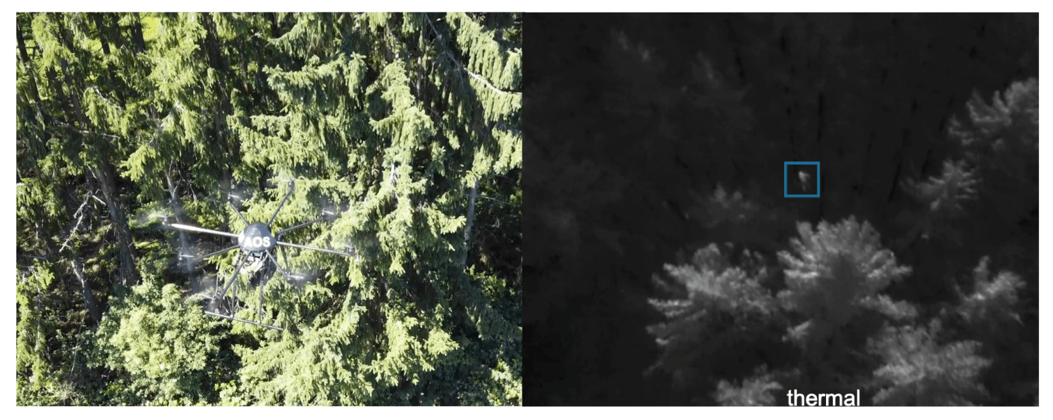
In 2018, a total of 2292 alpine search-and-rescue (SAR) operations were performed by ÖAMTC air emergency helicopters in Austria. Rescuing, lost, ill or injured persons often involves searching densely forested terrain. Sunlight is mostly blocked by trees and other vegetation, and the forest ground reflects little light. Thermal imaging systems are therefore employed to visualize the temperature difference between human bodies and the surrounding environment. Autonomous unmanned drones, that use AI to automatically detect people, will increasingly replace manned helicopters in future SAR operations as they offer higher flexibility at lower cost. However, such search missions remain challenging due to occlusion and high heat radiation by trees under direct sunlight.
In this project, we built and trained a recurrent convolution neural net (RCNN) to detect humans in thermal images shot by autonomous drones flying over densly forested, and therefore highly occluded, terrain.
The data
The data was captured by Schedl et al – see also their paper on this topic. The training and test data consisted of several sequences of thermal images shot in a total of 18 drone flights in close proximity to Linz, Austria. Twelve flights were performed above forests of various vegetation types, while the remaining six flights recorded data from above a meadow without any high vegetation. Each sequence consisted of somewhere between 26 and 71 images of size 640 x 512 and contained from zero up to about a dozen people. Additionally, we were given the absolute position of the drone and the camera parameters (the poses) for each of the images.
The recorded data was split into a training and a test set. The training data consisted of a total of 99 sequences and the test data contained 61 sequences. In each sequence, the locations of the people in the middle image were marked by hand. The following figure shows a few images of one of the training sequences, where we have overlayed the corresponding labels in the middle image.

Preprocessing and data augmentation
As data preprocessing steps, we first reduced the size of the images to 227 x 227. This drastically reduced memory consumption and sped up training. Additionally, we also used the known camera parameters to undistort the images. Finally, to alleviate training and to avoid saturated activations, we normalized the images to have zero mean and standard deviation one. As another preprocessing step, we also computed from the absolute poses the poses relative to the middle image. This also helps with training.
Since our training dataset was relatively small, we applied several data augmentation techniques. First, we flipped the images in each sequence once in horizontal, once in vertical, and once both, in horizontal and in vertical, direction – of course, in doing so, we also had to flip the relative poses and the labels accordingly. In this way, we could quadruple the number of training sequences from 99 to 396. As a second data augmentation method, we added subsequences of the original data, where we for example removed every second image. These methods yielded a training dataset of 1188 image sequences in total. Furthermore, we also clipped all sequences around the middle image to be of length 11 – 19. This again sped up training and allowed us to do more training epochs.
The following illustration summarizes our data preprocessing and augementation steps.

The preprocessed 227 x 227 image sequences together with the relative poses were then the input to our model and the locations of the people in the middle image were the targets we were trying to predict.
Model architecture
The model we used for this task was a recurrent convolutional neural network (RCNN). The idea of such a network is to capture spatial information (hence, the term “convolutional” in RCNN) as well as temporal information (this is where the “recurrent” comes from) in the data. In the literature, one typically finds two different kinds of RCNNs. The first approach uses a convolutional neural network (CNN) with recurrent convolutional filters to process information in spatial and temporal dimension simultaneously. The second approach uses a conventional CNN as feature extractor first, which is then followed by a recurrent neural network (RNN). Hence, in the second approach the data is first processed in spatial dimension and afterwards in temporal dimension. In our project, we followed the second approach, i.e. our model consisted of a CNN followed by an RNN. The main reason for choosing this approach over the CNN with convolutional filter was simply a matter of less work.
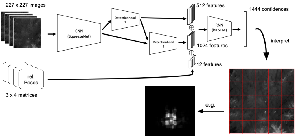
In particular, our model consisted of the well-known CNN SqueezeNet as a feature extraction network, followed by two detection heads that operate at different scales and consist of further convolutional layers, followed by ReLU activations and batchnormalization layers and a final fully connected layer paired with tanh activation. The input to the CNN was the sequence of images and the output of the two detection heads were sequences of feature vectors of length 512 and 1024, respectively.
These two sequences of feature vectors and the relative poses were then concatenated to give a sequence of feature vectors of length 1548. These feature vectors were then fed into an RNN consisting of a batchnormalization layer, a biLSTM layer with ReLU activation and a dropout layer for further regularization. This was followed by a final fully connected layer with sigmoid activation to give an output vector of size 1444.
Each of these 1444 outputs was then assigned to a fixed area of the middle image, in which we were trying to detect the people, and could be interpreted as the model’s confidence that this certain area contains a person. In this way, the task of object detection becomes in fact a classification task, in which we try to classify each area of the image on whether it contains people or not.
The following image illustrates our model and how its output is intepreted. Each output is assigned to one of the red grid cells (this grid is basically a hyperparameter that has to be fixed before training – in our case, it was set such that each grid cell was of size 6 x 6). In this way, the output of the model can be interpreted as a heatmap. The brighter the area, the more certain the model is that this area contains people.
Training
As already mentioned, by predicting the confidences for each area in the image, we were dealing with a classification task – in fact, a binary classification task. Hence, we used binary cross entropy as a loss function.
Unfortunately, our training could only be done on a single CPU. So, the number of epochs we could do in a reasonable amount of time was rather restricted. After a total of about 15 epochs (which still took ages) with a minibatch size of 32 and a learning rate which dropped from 10-3 to 10-4, we obtained our final model.
Results
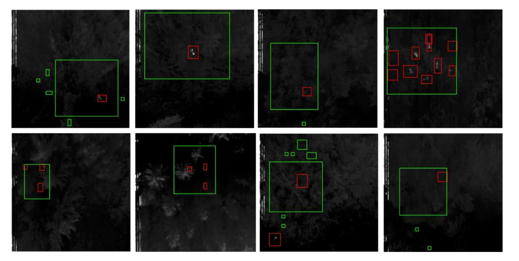
Before we could evaluate our model, we first had to transform its outputs into actual predictions of bounding boxes. To this end, we considered each grid cell as a possible candidate for a prediction and applied a technique similar to non-maximum suppression (check out this article for further information on NMS). First, we removed all candidates with very low confidence. In our case, the threshold for this was 2,5%. Then, neighbouring candidates were successively merged to give the final predictions. Here are some exemplary predictions of our model – the red rectangles are the real labels and the green rectangles are the predictions of the model.
Evaluating our model on the 61 sequences from the test data, which were also preprocessed as the training data but of course not augmented, yielded 37 out of 53 possible detections, an average precision of 56% and a total of 204 false positives. Note that we count a prediction as correct whenever there is an overlap with a label but we only count at most one prediction per label. In the following, we also show the corresponding precision-recall curve.
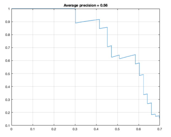
As can be seen, while we could actually detect quite a reasonable amount of people, we suffered from a lot of false positives. So, apparently our model does not have the terminator’s intelligence but at least it is also not a complete Neanderthal. We record this as a success!

All code needed to reproduce our results is provided in this github repository.
